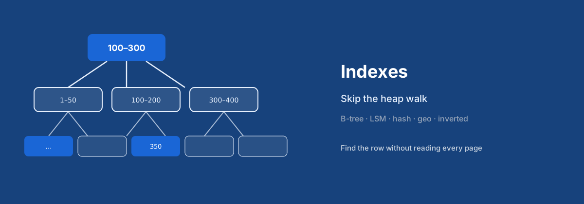
Why indexes show up in interviews
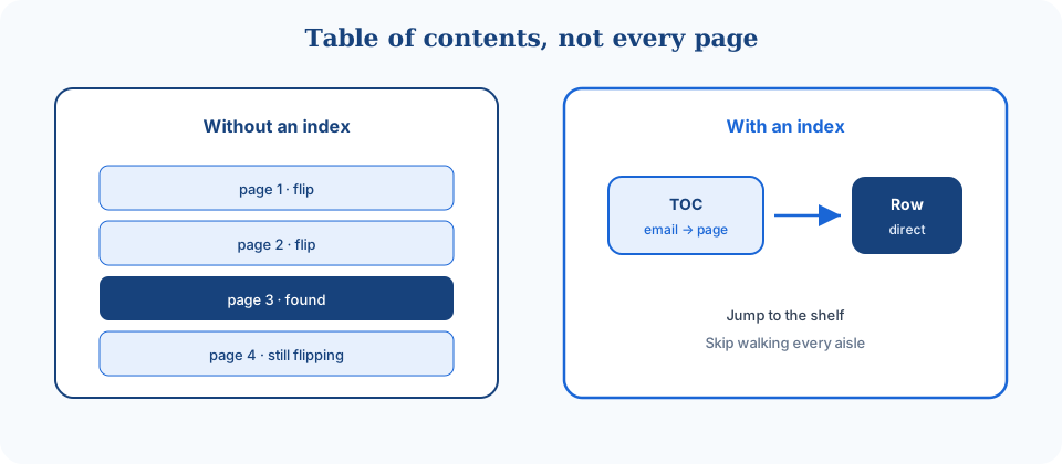
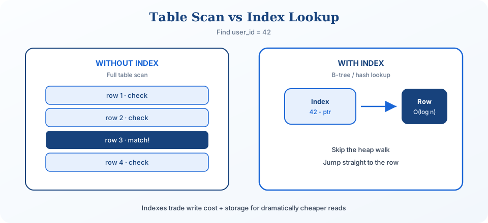
Search a user’s profile by email in a table with millions of rows. With no index, the database walks the heap sequentially — every page loaded, every row checked — until it finds a match. That’s the library problem: reading every book on every shelf to find one title.
B-tree for equality and ranges.
LSM-style primary storage (Cassandra, RocksDB).
Geohash or R-tree — not two 1D indexes.
Inverted index — LIKE '%x%' won’t cut it.
We’ll cover how indexes sit on disk, the cost model, then the types that actually appear on whiteboards: B-trees, LSM trees, hash indexes, geospatial (geohash / quadtree / R-tree), inverted indexes, and the optimization patterns — composite and covering.
How database indexes work
Table data usually lives in a heap file — rows appended in no particular order, like a notebook filled as entries arrive. Indexes are separate structures that map searchable keys to those row locations (or to the leaf pages that hold them).
Data lives on disk (usually SSDs). CPUs only work on what’s in RAM. A query without an index may load millions of pages to find one row. Prefetch and buffer pools help, but sequential full scans still lose to a short indexed path.
With an index, you follow a structured path to the pages that matter — table of contents instead of every page. Random access is still slower than sequential access even on SSDs (the gap is smaller than HDDs, not zero). For large datasets, that difference is why indexing stays critical.
The cost of indexes
Indexes aren’t free. Each one takes disk space — sometimes a large fraction of the table. Every insert or update must maintain the heap and every index on those columns. More indexes → more write amplification.
- Write-heavy, rarely read — logging / audit tables: index overhead often isn’t worth it.
- Tiny tables — a few hundred rows: a sequential scan can beat index traversal.
- Unused indexes — monitor usage; drop the ones that never show up in plans.
Memory pressure from “too many indexes” is often overstated — buffer pools are smarter than textbook diagrams. The real discipline is: index the queries you run, not every column that looks searchable.
Types of indexes (the interview set)
Production databases ship exotic index types you’ll rarely touch. Interviews care about a short list: B-tree (default), LSM as a storage/index story for write-heavy systems, hash for exact match, geospatial for nearby points, inverted for text.
B-tree indexes
B-trees are the default index in relational databases. They’re a self-balancing tree of sorted keys that keeps lookups, inserts, and deletes predictable as data grows. Unlike a binary tree (two children), a B-tree node holds many keys — often hundreds — so tree height stays tiny.
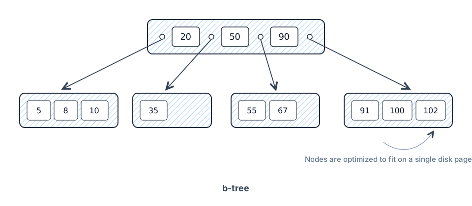
- All leaf nodes sit at the same depth.
- A node holds roughly m/2 to m keys (m = order).
- k keys → k+1 children; keys inside a node stay sorted.
- Leaves point at heap tuples (or hold the row in clustered / index-organized designs).
That layout maps to how databases read disk: one node ≈ one page. PostgreSQL’s primary keys, unique constraints, and most secondary indexes are B-trees (practically B+ trees — data in leaves). MongoDB indexes the same way. DynamoDB sorts items within a partition by sort key for range queries; its engine is widely understood as LSM-style storage, not a classic B-tree table file.
CREATE TABLE users (
  id SERIAL PRIMARY KEY,
  email VARCHAR(255) UNIQUE
);
-- Postgres: B-tree on id (PK) and on email (UNIQUE)
Why they’re the safe interview answer: sorted order (ranges + ORDER BY), self-balancing, equality and ranges, disk-friendly fanout. If you’re unsure which index to propose, say B-tree.
LSM trees (Log-Structured Merge Trees)
B-trees update pages in place. At tens or hundreds of thousands of writes per second, random leaf updates become the bottleneck. LSM trees flip the model: buffer in memory, append sequentially to disk, merge in the background.
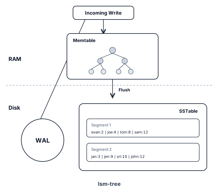
- Memtable — sorted structure in RAM (skip list / tree).
- WAL — sequential append for durability.
- Flush — frozen memtable becomes an immutable SSTable (big sequential write).
- Compaction — merge SSTables, drop tombstones and duplicates.
Reads pay for that write speed. A point lookup may check the memtable, pending flushes, then several SSTables (newest first). Mitigations: bloom filters (skip definite misses), sparse indexes (skip blocks outside the key range), and compaction strategy (size-tiered vs leveled). How bloom filters work as probabilistic membership structures: Specialized data structures.
Interview cue: write ≫ read — metrics ingest, audit logs, IoT telemetry — LSM-backed stores (Cassandra, RocksDB, DynamoDB-style) are the right story. User-facing pages with many point reads per request usually stay on B-tree engines unless you’ve measured otherwise. How LSM + compression + time partitions combine for metrics: Time-series databases.
Hash indexes
Hash indexes are a persistent hashmap: key → bucket → row pointer. Average lookup is O(1). Collisions use chaining / overflow pages. They do not preserve order — no ranges, no sorting help.
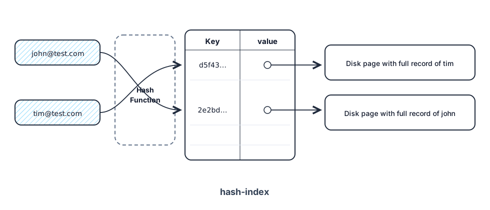
In practice they’re rare on disk-backed OLTP. PostgreSQL supports hash indexes but defaults to B-trees — equality is almost as fast, and you keep ranges. Hash shines more for in-memory stores (Redis key lookups; MySQL MEMORY historically defaulted to hash).
Geospatial indexes
Location questions (Uber, Yelp, “find nearby X”) show up more in interviews than in most day jobs. The trap: indexing latitude and longitude separately with two B-trees.
CREATE INDEX idx_lat ON restaurants(latitude);
CREATE INDEX idx_lng ON restaurants(longitude);
-- Looks sensible. Falls apart for “within 5 miles of me.”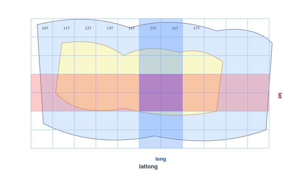
A latitude range is a band around the globe; intersecting with longitude still yields a fat rectangle you must filter. You need an index that understands 2D proximity. Three approaches interviewers expect you to name: geohash, quadtree, R-tree. Master the problem statement and one solution deeply; you don’t need production PostGIS expertise unless the role is geo. Full deep dive: Proximity search.
Geohash
Encode lat/lng into a base32 string so nearby points usually share a prefix. Longer string → finer cell. Index the string with a normal B-tree and do prefix / adjacent-cell scans for radius queries.
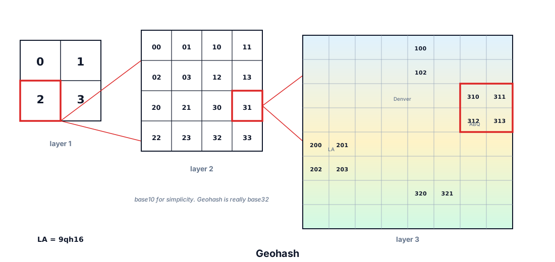
Edge case: points on opposite sides of a cell boundary can have distant prefixes even when physically close — query neighboring cells. For interviews, geohash is the cleanest story if you only remember one geo approach.
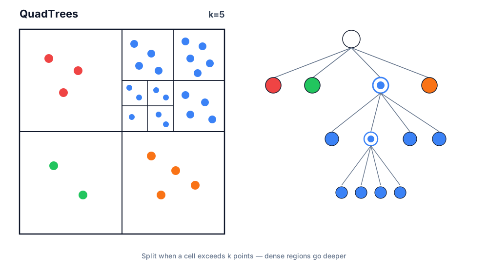
Quadtree
Recursively split space into four equal quadrants when a cell gets too dense. Adaptive resolution; needs a specialized tree. Less common as a primary DB index today; the subdivision idea feeds R-trees and map-tile pyramids.
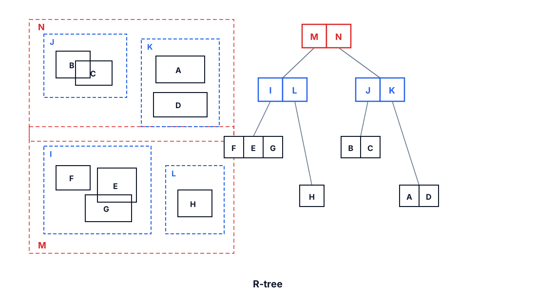
R-tree
Hierarchy of flexible, overlapping bounding rectangles that fit the data — not a fixed grid. Handles points and polygons in one structure. Default spatial index in PostGIS / MySQL spatial. Overlap can force multi-branch searches; implementations tune that against disk I/O.
Inverted indexes
WHERE content LIKE '%database%' can’t use a B-tree — the match can sit anywhere in the string. The engine falls back to scanning text. An inverted index flips the relationship: term → list of documents (like a book’s back-of-book index).
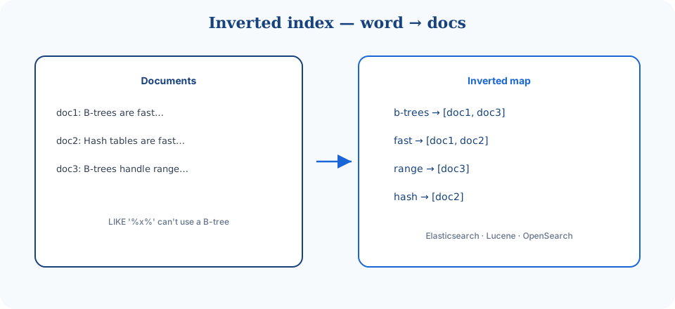
b-trees  → [doc1, doc3]
fast     → [doc1, doc2]
range    → [doc3]
hash     → [doc2]
Production search (Elasticsearch, Lucene, OpenSearch) adds analysis: tokenize, lowercase, drop stop words, stem. Then scoring, fuzzy match, phrase queries. Cost: storage and update fan-out when documents change. For rich text search, that’s the trade you accept — often via CDC from the primary DB into a search cluster. See Elasticsearch for the full deep dive and Key technologies for where search sits in the stack.
Index optimization patterns
Picking a type is half the job. The other half is matching indexes to real access patterns — query plans, not vibes.
Composite indexes
One B-tree on multiple columns in a fixed order beats intersecting two single-column indexes for common multi-filter queries.
-- Feed-style query
SELECT * FROM posts
WHERE user_id = 123
  AND created_at > '2024-01-01'
ORDER BY created_at DESC;

-- Prefer one composite:
CREATE INDEX idx_user_time ON posts(user_id, created_at);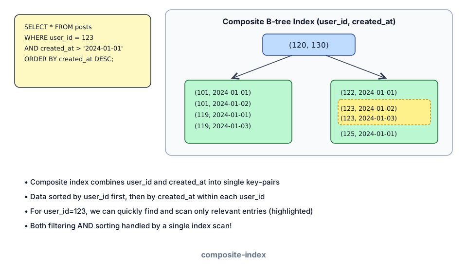
Order matters. (user_id, created_at) helps queries that lead with user_id. It does little for WHERE created_at > … alone — B-trees use leftmost prefixes. Selectivity matters, but query shape often wins: if you always sort by time within a user, put time second even if it’s less selective.
- Order history:
(customer_id, order_date) - Event processing:
(status, priority, created_at) - Activity feeds:
(user_id, type, timestamp)
Covering indexes
A covering index includes every column the query needs so the engine can answer from the index alone — no heap fetches for like counts on a feed row.
CREATE INDEX idx_user_time_likes
  ON posts(user_id, created_at) INCLUDE (likes);
-- Postgres: INCLUDE keeps likes out of the sort key but in the leafIndex selection drills
Anti-patterns
- Indexing low-cardinality columns alone (boolean).
- Functions on column in WHERE without expression index.
- Over-indexing write-heavy tables "just in case."
Failure modes to mention
Call out at least one dependency failure (DB down, cache stampede, queue lag, region outage) and your mitigation (timeouts, retries with jitter, degraded mode, circuit breaker).
Cost and performance levers
Interview Q&A by level
Practice saying these out loud for database indexing. Interviewers grade clarity and judgment more than buzzwords.
Match depth to the bar: define → trade off → operate. Don't dump principal answers in an entry-level screen.
Wrapping up
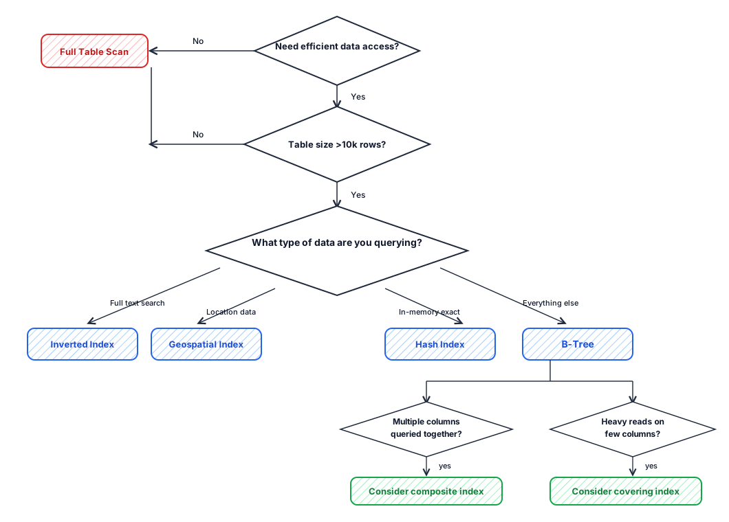
- Index columns you filter and sort on — tie them to APIs you already drew.
- When unsure of type: B-tree.
- Nearby points: geospatial (learn geohash; bonus if you contrast R-trees).
- Full-text: inverted index / search engine — not
LIKE '%…%'. - Write-dominated primary store: LSM story, not “add more B-trees.”
Pair this with data modeling — schema without indexes is half a design — and Scaling reads for how indexes sit in the full read ladder. On the whiteboard, name the hot query and the index that serves it, then move on.
How to answer this in a backend interview
Before I add indexes I'd write the hottest queries. For 'orders by user_id then created_at desc' that's a composite (user_id, created_at). Equality columns go left; range and sort follow. I'd consider a covering index only if the napkin math says we're table-scanning a hot path. Writes pay for every index, so I won't index every filterable column. Finally I'd mention EXPLAIN / slow-query logs as how we'd validate in production — not as a design substitute.
Related Lattice posts: Data modeling · PostgreSQL · Scaling reads · Sharding