Patterns that make TSDBs hum
In this deep dive we cover the patterns that enable high-throughput time-series databases. The ideas together make TSDBs hum, but each has wider applicability to distributed systems — especially infra-style interviews. None are terribly complex; the magic is in how you put them together.
Append-only · LSM · WAL.
Δ / Δ-of-Δ · XOR floats.
By time · drop old chunks.
Bloom · rollups · tag index.
A motivating example
Design a monitoring system for a cloud provider: 100,000 servers, each emitting 5 metrics every 10 seconds (CPU, memory, disk I/O, network). That's 50,000 metrics/second — ~4.3 billion points/day. Users need dashboards, alerts, and week-long debug queries.
CREATE TABLE metrics (
    timestamp TIMESTAMP,
    host VARCHAR(255),
    metric_name VARCHAR(255),
    value DOUBLE PRECISION
);
At 4.3B rows/day you're at ~30B rows/week. Even with indexes, "average CPU for host-42 over the past hour" crawls. Write throughput (50k+/s with bursts) crushes a single Postgres. Storage waste: full host and metric names repeated → 50–100 bytes/point when the payload is really a timestamp + float (~16 bytes).
InfluxDB, TimescaleDB, Prometheus, and peers are built for this. Here's how.
Append-only storage
First insight: if you write a lot, don't update in place — always append to the end of a file.
Traditional updates: find the row → read → modify → write back. That's random I/O. HDDs seek at ~100–200 ops/s; even SSDs prefer sequential patterns.
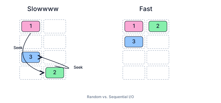
How do you organize for reads if you only append? Enter LSM trees.
LSM trees
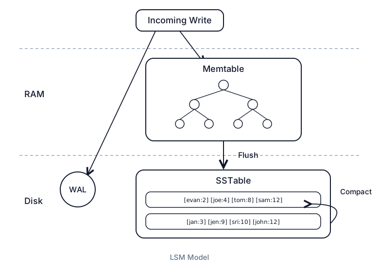
LSM trees power high-write stores including InfluxDB, Cassandra, and LevelDB. Same idea as Database indexing / Cassandra: turn random writes into sequential writes, reorganize in the background.
- Write to memory (memtable) — sorted structure (skip list / tree) in RAM. Sorted so flushes produce sorted files for binary search, range scans, and merge-sort compaction.
- Flush to disk (SSTable) — when full, sequential write of an immutable Sorted String Table; clear memtable.
- Background compaction — merge SSTables, drop duplicates and tombstones so reads don't check forever-growing file sets.
Delta encoding and compression
Time-series data has a unique property: adjacent values are often similar. CPU at 45.2%, 45.3%, 45.1% — storing full floats wastes space.
Delta encoding stores differences. Combined with varint, tiny deltas take 1–2 bytes instead of 8.
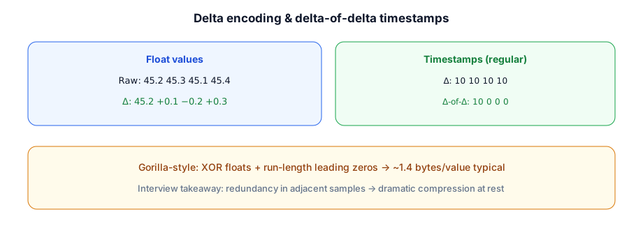
- Timestamps — delta-of-delta; perfectly regular series compress toward ~1 bit/value (Facebook Gorilla).
- Floats — XOR similar values → mostly zeros → store first differing bit + meaningful bits (~1.37 bytes/value typical).
Time-based partitioning
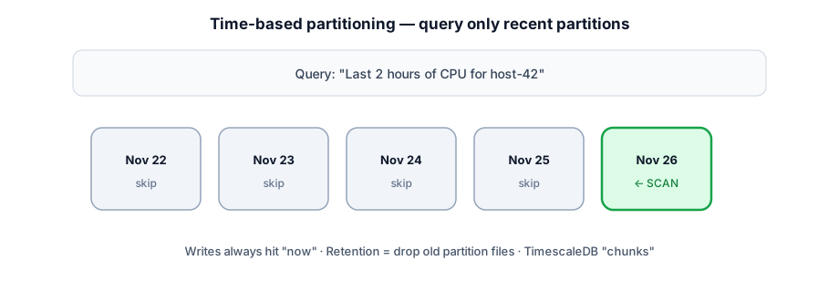
Group data into partitions by time window (day/week). Partitions may live on one machine or many.
- Writes localize — all new data hits the "now" partition.
- Reads prune — "last hour" only opens recent partitions.
- Retention is trivial — drop partitions older than N days; no massive DELETE scans.
Bloom filters for read optimization
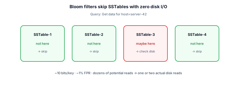
LSM means many SSTables. Point lookups across a long time range for one host could touch dozens of files. Bloom filters answer "definitely not here" vs "maybe" with zero disk I/O.
Downsampling and rollups
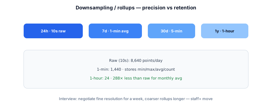
Raw 10-second metrics are great for recent debug; nobody needs that for last year's dashboards. Downsampling reduces resolution of older data.
Block-level metadata
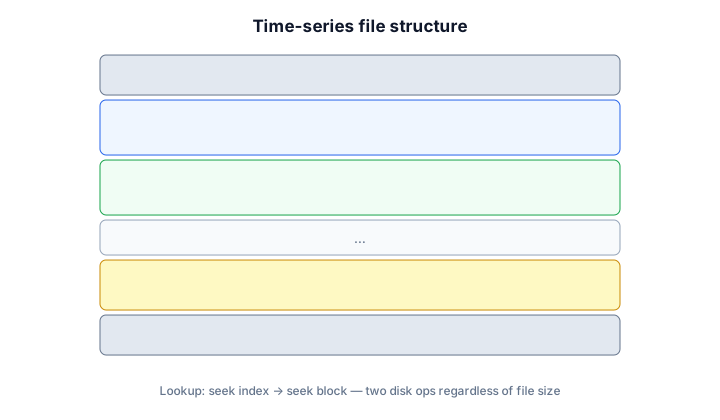
Like query planning in Elasticsearch, TSDBs keep per-block min/max timestamps (and often values). Query "CPU > 10%" skips a block whose max is 5% — no read. Combined with time partitions, another pruning layer as data grows.
Putting it together
Data model
- Measurements / metrics — like tables (
cpu_usage). - Tags — indexed metadata for filtering (
host,region). - Fields — actual measured values (not indexed).
- Timestamps — when measured.
cpu_usage,host=server-1,region=us-west value=45.2 1699999200000000000
└──────── measurement + tags ────────┘ └──field─┘ └──── timestamp ────┘Storage engine
- WAL — durability before crash recovery.
- In-memory buffer — memtable by measurement + tags.
- Flush — compressed immutable files.
- Compaction — merge files, drop deletes.
Query execution
SELECT mean(value) FROM cpu_usage WHERE host='server-1' AND time > now()-1h GROUP BY time(5m)
- Identify partitions overlapping the time filter.
- Locate series via in-memory tag index.
- Read memtable + relevant disk files; merge.
- Stream aggregations — don't load everything into RAM first.
Key insight: exploit time locality (recent data hot) and series locality (points for one series co-located) to minimize disk access.
Worked example: multi-tag query
Ingest a few points across hosts/regions. Each unique measurement + tags combo is a series. Data for each series lives in compressed blocks; an inverted tag index (like Elasticsearch) maps tag values → series IDs.
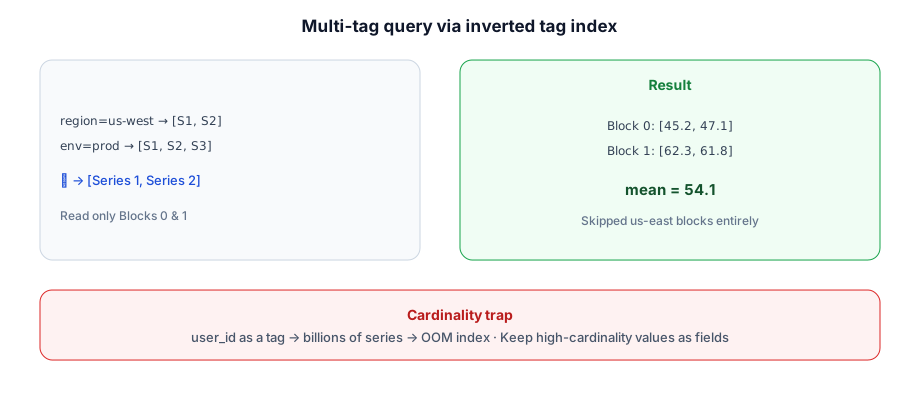
Query region=us-west AND env=prod: intersect postings → Series 1 & 2 → Blocks 0 & 1 only → mean = 54.1. Compared to Postgres row scatters across disk, series-oriented storage keeps needed values physically co-located — writes optimized to help reads.
Where things break: cardinality
Cardinality = unique tag combinations. 1,000 hosts × 50 metrics = 50,000 series — fine. Add user_id with 10M users → potential hundreds of billions of series.
TSDBs keep an in-memory index of all series. Billions of series → OOM; queries crawl. High-cardinality values (user IDs, request IDs) belong as fields, not tags — you can write them but lose TSDB read advantages.
In your interview
What to say out loud
"I'd stretch Postgres or DynamoDB first. If we're at tens of thousands of samples/sec with time-range dashboards and retention, I'd use a TSDB pattern: append-only LSM ingest, time partitions for retention, tags for host/region only — never user_id as a tag — and negotiate downsampling for older data. Prometheus or TimescaleDB depending on ops preference."
- Name the write problem (random I/O) before naming Influx/Prometheus.
- Call out cardinality explicitly when tagging.
- Offer rollup negotiation without being asked.
- Don't invent a custom TSDB on the whiteboard — name the production default.
Cost and performance levers
Metrics path design
Cardinality bomb
High-cardinality labels (user_id on every metric) explode time series count. Prefer bounded label sets; use logs/events for high-cardinality debugging.
Failure modes to mention
Call out at least one dependency failure (DB down, cache stampede, queue lag, region outage) and your mitigation (timeouts, retries with jitter, degraded mode, circuit breaker).
Interview Q&A by level
Practice saying these out loud for time-series databases. Interviewers grade clarity and judgment more than buzzwords.
Match depth to the bar: define → trade off → operate. Don't dump principal answers in an entry-level screen.
Wrapping up
Time-series databases compose fundamental patterns — not exclusive to metrics:
- Append-only storage → sequential I/O
- LSM trees → high write throughput
- Delta / XOR compression → exploit redundancy
- Time partitions → localized writes + cheap retention
- Bloom filters → skip useless SSTable reads
- Downsampling → trade precision for historical efficiency
- Block metadata → prune during scans
Together: order-of-magnitude wins on the target workload. Millions of events/sec isn't magic — it's append-only logs, LSM, compression, Bloom filters, rollups, and careful data modeling.
Continue with Database indexing, Cassandra, Specialized data structures, PostgreSQL, and Key technologies.