Why Elasticsearch
Many system design problems involve search and retrieval: you've got a lot of "things" and you want to find the right one(s). Most databases handle this reasonably well — Postgres with a full-text index is sufficient for many problems — but at a certain scale or level of sophistication you'll want a purpose-built system with sorting, filtering, ranking, faceting, and more. Enter Elasticsearch.
From an interview perspective, this deep dive tackles two angles. First, you'll learn how to use Elasticsearch — a powerful tool for startup and product-architecture interviews where complex search questions come up. Second, you'll learn how it works under the hood. As a piece of distributed systems engineering, Elasticsearch brings together concepts useful even outside search — and some gnarly interviewers may ask you to pretend Elasticsearch doesn't exist and explain the top-level concepts yourself. That's more common for infra-heavy roles at cloud companies.
JSON docs · indices · mappings.
match · bool · nested · geo.
Lucene segments · inverted index.
CDC from Postgres · not primary DB.
Basic concepts
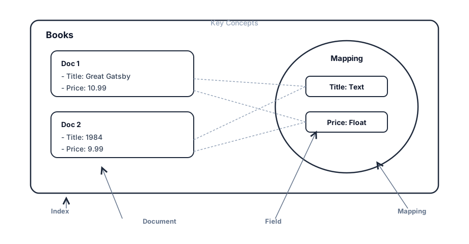
From a client perspective, the important concepts are documents, indices, mappings, and fields.
Documents
Documents are the individual units of data you're searching over. A "document" doesn't have to be a website or blog post — think of it as any JSON object. Like books in our bookstore:
{
  "id": "XYZ123",
  "title": "The Great Gatsby",
  "author": "F. Scott Fitzgerald",
  "price": 10.99,
  "createdAt": "2024-01-01T00:00:00.000Z"
}
Indices
An index is a collection of documents. Each document has a unique ID and a set of fields (key-value pairs). Think of an index as a database table. Searches happen against indices and return matching documents.
Note: this overloads the general term "index" (auxiliary data structures that make lookups faster). We'll clarify which meaning we're using.
Mappings and fields
A mapping is the schema of the index — field names, data types, and how each field is processed and indexed. You can put arbitrary data in a document, but the mapping determines which fields are searchable:
{
  "properties": {
    "id": { "type": "keyword" },
    "title": { "type": "text" },
    "author": { "type": "text" },
    "price": { "type": "float" },
    "createdAt": { "type": "date" }
  }
}
keyword treats the whole value as one token — efficient for exact lookups and sorting (hash-table style). text is tokenized for full-text search (inverted-index style). Types can be arbitrarily complex: nested objects, arrays, geo_point, geo_shape, custom analyzers, even embeddings for semantic search.
Basic use
Elasticsearch exposes a clean REST API. Here's the essential lifecycle: create an index, set a mapping, add documents, search.
Create an index
PUT /books
{
  "settings": {
    "number_of_shards": 1,
    "number_of_replicas": 1
  }
}
Set a mapping
When dynamic mapping isn't appropriate — maybe most fields aren't searchable — define the schema up front:
PUT /books/_mapping
{
  "properties": {
    "title": { "type": "text" },
    "author": { "type": "keyword" },
    "description": { "type": "text" },
    "price": { "type": "float" },
    "publish_date": { "type": "date" },
    "categories": { "type": "keyword" },
    "reviews": {
      "type": "nested",
      "properties": {
        "user": { "type": "keyword" },
        "rating": { "type": "integer" },
        "comment": { "type": "text" }
      }
    }
  }
}
The nested review field is a fair interview trade-off question. If reviews are infrequently updated and frequently queried with the book, nesting can be efficient. Otherwise, a separate reviews index is often better — the same normalization vs denormalization tension you know from SQL.
Add documents
POST /books/_doc
{
  "title": "The Great Gatsby",
  "author": "F. Scott Fitzgerald",
  "description": "A novel about the American Dream in the Jazz Age",
  "price": 9.99,
  "publish_date": "1925-04-10",
  "categories": ["Classic", "Fiction"],
  "reviews": [
    { "user": "reader1", "rating": 5, "comment": "A masterpiece!" },
    { "user": "reader2", "rating": 4, "comment": "Beautifully written, but a bit sad." }
  ]
}
Each response includes a document ID and metadata about persistence — including _version, used for optimistic concurrency control on updates.
Updating documents
Full document replace via PUT /books/_doc/{id} works but risks overwriting concurrent edits. Guard with ?version=1 so the update only succeeds if the version matches — clients retry on conflict.
Partial updates via POST /books/_update/{id} with a doc payload avoid fetching the whole document. In a distributed, asynchronous system, being explicit about update semantics matters — good fodder for API design questions.
Search
Query syntax is JSON-based and feels closer to structured search than raw SQL. Simple match on title:
GET /books/_search
{
  "query": {
    "match": { "title": "Great" }
  }
}
Combine constraints with a bool query — title contains "Great" and price ≤ 15:
{
  "query": {
    "bool": {
      "must": [
        { "match": { "title": "Great" } },
        { "range": { "price": { "lte": 15 } } }
      ]
    }
  }
}
Search inside nested reviews — books with an "excellent" review and rating ≥ 4:
{
  "query": {
    "nested": {
      "path": "reviews",
      "query": {
        "bool": {
          "must": [
            { "match": { "reviews.comment": "excellent" } },
            { "range": { "reviews.rating": { "gte": 4 } } }
          ]
        }
      }
    }
  }
}
Results include _score (relevance, default TF-IDF family), document IDs, and _source unless you project fields away. You're applying mapping constraints to indexed data — the engine never has to scan every document in the cluster for a token lookup.
Geospatial search
For Yelp, Uber, or any location-based service, Elasticsearch's native geo support is a strong interview answer compared to bolting lat/lng onto a relational DB. Two primary field types: geo_point (single lat/lon) and geo_shape (polygons, lines, delivery zones).
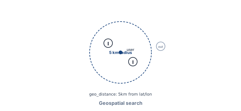
geo_distance — restaurants within 5 km, combinable with cuisine and rating filters.{
"query": {
"geo_distance": {
"distance": "5km",
"location": { "lat": 40.7128, "lon": -74.0060 }
}
}
}Under the hood, geo_point uses BKD trees (k-d tree variants optimized for block storage) to narrow the 2D search space efficiently — not separate B-trees on latitude and longitude. See Proximity search for the full trees-vs-encoded-keys story, and Database indexing for the broader index menu.
Sort and pagination
Sort
Explicit sort overrides default relevance ordering. Sort by price ascending, or by nested review rating with mode: max. Custom script sorts (Painless) exist for computed values — use sparingly; they don't come free.
With no sort specified, results order by _score (TF-IDF-related by default). Worth 10 minutes to understand TF-IDF — it shows up far beyond search.
From/size
The simplest pagination: from (offset) and size (page length). Fine for early pages; deep pagination (beyond ~10k) forces the cluster to sort and discard all preceding hits on every request — expensive.
Search after
For deep pagination, pass the sort values of the last result as search_after. Each page only fetches what comes after the cursor — efficient, but forward-only (no random page jumps) and client must remember state.
{
  "size": 10,
  "sort": [{ "date": "desc" }, { "_id": "desc" }],
  "search_after": [1463538857, "654323"]
}
Point in time (PIT) cursors
When the index mutates during pagination, search_after alone can skip or duplicate rows. PIT + search_after freezes a consistent view: create a PIT, paginate with search_after, close the PIT when done. More overhead, but stable cursors across long result walks.
How it works
Elasticsearch is a high-level orchestration layer on Apache Lucene — the optimized low-level search library. Elasticsearch handles distributed coordination, APIs, aggregations, and near-real-time refresh; Lucene is the heart of indexing and retrieval.
Cluster architecture
A cluster is multiple nodes, each configured for one or more roles:
- Master — cluster admin: create/delete indices, node membership. One active master via leader election among master-eligible nodes.
- Data — stores shards; query and fetch phases run here.
- Coordinating — receives client requests, plans queries, fans out to shards, merges results.
- Ingest — optional transforms on the write path.
- ML — machine learning tasks.
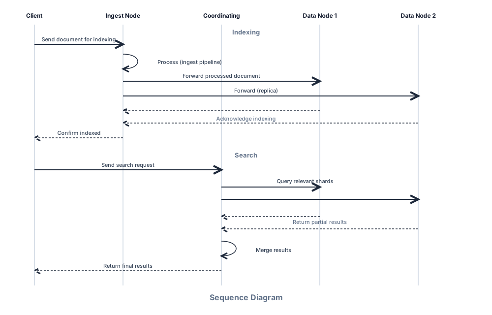
Data nodes can be tiered hot/warm/cold/frozen by query likelihood and mutability. Ingest and coordinating nodes are often colocated in smaller clusters; large deployments dedicate hosts by workload (CPU-bound ingest vs I/O-heavy data).
Data nodes, shards, and replicas
Data nodes separate raw _source JSON from Lucene indexes used for search — like a document store plus specialized indexes. Queries run in two phases: query (identify matching doc IDs via index structures) and fetch (optionally load _source). Ideal queries never touch source at all.
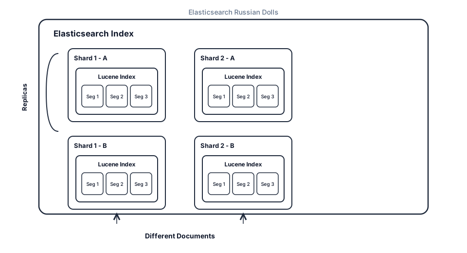
Shards split an index across hosts for horizontal scale. Searches hit all relevant shards in parallel; the coordinating node merges and sorts. Replicas are exact shard copies — high availability and read throughput. If one primary handles X queries/sec, Y replicas can roughly multiply read capacity (all else equal). Coordinating nodes load-balance across primary and replica copies.
One Elasticsearch shard maps 1:1 to one Lucene index. Many shard operations (merge, refresh, search) are proxy operations on Lucene underneath — oversimplify to "availability and scale on top of a bag of Lucene indexes" and you're not far off.
Lucene segments
Lucene indexes are built from segments — immutable containers of indexed data. Writes batch into new segments; when segments multiply, background merges combine them. Deletes don't erase data immediately: each segment tracks deleted doc IDs and hides them at query time; merges eventually purge tombstones.
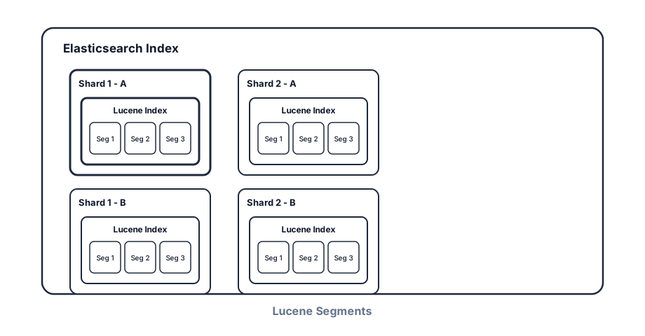
- Immutability → fast writes (append-only), safe caching, simpler concurrent reads.
- Trade-off → segment merges, temporary storage bloat, write-heavy workloads struggle.
- Interview lesson → immutability at the right layer is a recurring infra pattern.
This is part of why Elasticsearch isn't a great primary store for rapidly mutating data — updates pay merge and tombstone tax. Pair it with a write-optimized source of truth and accept eventual consistency on the search side.
Inverted index and doc values
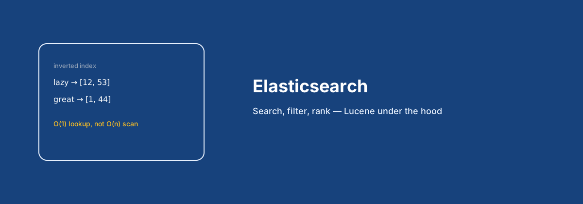
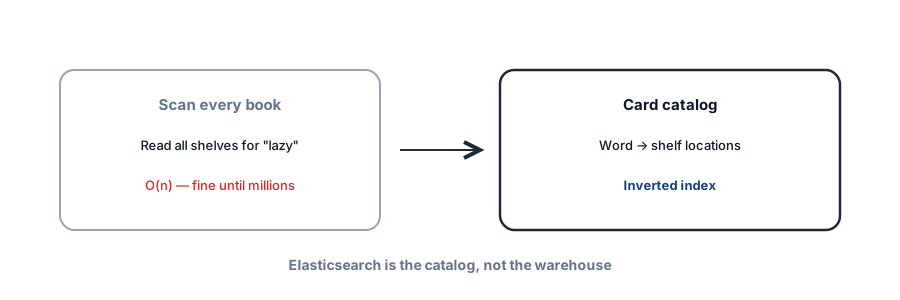
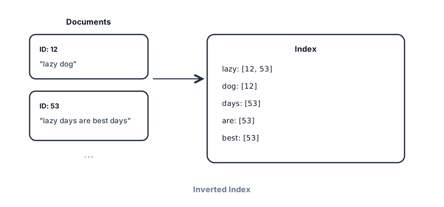
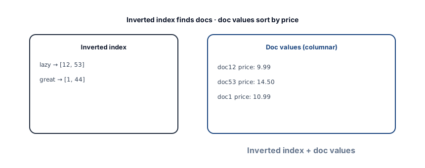
If Lucene is the heart of Elasticsearch, the inverted index is the heart of Lucene. To find things fast you either organize data for your access pattern, or copy data and organize the copy. With a billion books, scanning every title for "lazy" is O(n). An inverted index maps "lazy" → [doc12, doc53] for O(1) lookup.
Doc values answer the next question: how do we sort matched docs by price? Row-oriented stores read whole rows to reach one column. Doc values store each field columnar — contiguous per-field arrays across documents in a segment — so sorting and aggregations read one column at a time, Spark/Redshift style.
Coordinating nodes and query planning
Coordinating nodes parse queries and run a query planner — deciding whether to use an inverted index, in what order to intersect posting lists, and how to merge shard results.
Example: search "bill nye". "bill" might match millions of docs; "nye" hundreds. Intersect the smaller set first, then verify phrase match — orders of magnitude faster than the reverse. Elasticsearch keeps field statistics (cardinality, popularity) to pick plans dynamically. Same family of idea as SQL optimizers: statistics + indirection so performance adapts to the data.
In your interview
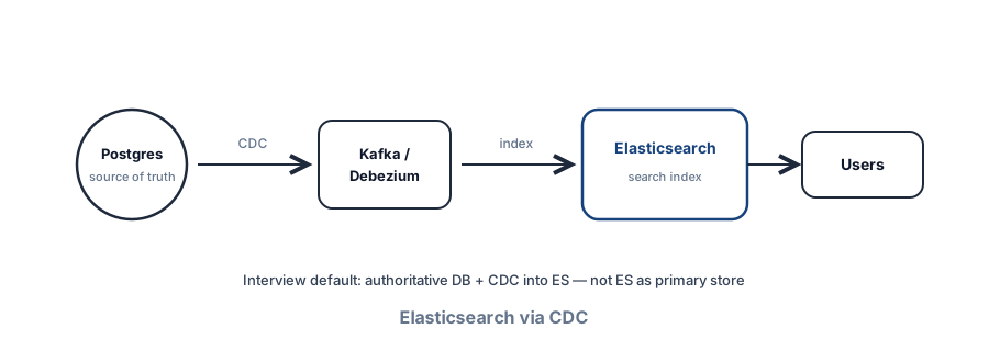
Elasticsearch fits any design with complex search — usually via CDC from Postgres, DynamoDB, or similar. Say the CDC sentence before the interviewer asks where data comes from.
- Not your database — search engine first; durability and consistency history mean keep authoritative data elsewhere.
- Read-heavy — write-heavy counters (likes, impressions) will hurt; buffer writes or use another store.
- Eventual consistency — results can be stale; say whether that's acceptable.
- Denormalize — not relational; aim for one or two queries to render a result page.
- Not always needed — under ~100k docs, Postgres GIN full-text may suffice. See Key technologies.
- Sync failures cause drift — design retry, idempotent indexing, and monitoring.
Lessons from Elasticsearch
- Immutability at the right layer unlocks caching, compression, and simpler concurrency — segments are the textbook example.
- Separate query execution from storage — coordinating vs data nodes optimize different paths.
- Tailored data structures (inverted index, doc values, BKD trees) beat generic indexes for specific access patterns.
- Distributed scale adds CAP trade-offs — replicas and partitions buy throughput and fault tolerance at the cost of consistency complexity.
Cost and performance levers
Search design sketch
Indexing pipeline
Postgres → CDC (Debezium) → Kafka → indexer → ES. Reindex with aliases for zero-downtime mapping changes. Never dual-write from app forever without a repair path.
Failure modes to mention
Call out at least one dependency failure (DB down, cache stampede, queue lag, region outage) and your mitigation (timeouts, retries with jitter, degraded mode, circuit breaker).
Interview Q&A by level
Practice saying these out loud for Elasticsearch. Interviewers grade clarity and judgment more than buzzwords.
Match depth to the bar: define → trade off → operate. Don't dump principal answers in an entry-level screen.
Wrapping up
Elasticsearch is enormous — we've covered client concepts, essential API flows, geo and pagination, and the Lucene/distributed machinery interviewers probe on infra loops. Use it when search complexity or scale outgrows your primary DB; justify the CDC pipe, mapping choices, and consistency model. For semantic similarity and RAG, see Vector databases. For the broader toolbox context, start with Key technologies; for inverted indexes in isolation, see Database indexing.