Why vector databases matter now
If you've been paying attention to tech over the past few years, you've noticed embeddings everywhere — search that understands intent, eerily relevant recommendations, chatbots retrieving from massive document collections. All rely on the same primitive: finding similar things, fast.
This isn't new — vector techniques powered recommendation systems for years. What's changed is modern ML amplifying the use cases: semantic search, RAG, multimodal similarity. Traditional databases excel at exact lookups (user ID 12345, orders on January 1st). Ask one to "find documents similar to this" and you're in trouble. That's where vector databases come in.
Fixed-length embedding vectors.
Top-K nearest neighbors.
HNSW · IVF · LSH (ANN).
Recall · latency · memory.
What's a vector anyway?
A vector (or embedding) is an array of numbers representing something — a word, sentence, image, user, product, anything you can feed an ML model. The magic: similar things get similar vectors.
"The cat sat on the mat"    → [0.12, -0.34, 0.78, ..., 0.45]  // 1536 dims
"A feline rested on a rug"  → [0.11, -0.32, 0.79, ..., 0.44]  // very close
"The stock market crashed"  → [-0.89, 0.12, -0.45, ..., 0.23] // far away
Typical embeddings have 128–1536 dimensions (OpenAI text-embedding-3-large uses 3072). Individual dimensions aren't human-interpretable — what matters is geometric relationships reflecting semantic relationships.
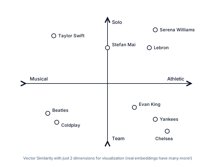
"Similarity" depends on the embedding model. Pre-trained models (OpenAI embeddings, Sentence Transformers, BERT, CLIP) capture broad semantic similarity — think of them as an expensive GPU function: data in, fixed-length vector out. Custom models target precise similarity — e.g. "frequently bought together" where diapers and bottles are profoundly similar to new parents but only vaguely similar semantically.
Similarity metrics
Once you have vectors, you need a way to measure closeness:
- Euclidean distance (L2) — straight-line distance in space. Smaller = more similar. Cares about direction and magnitude.
- Cosine similarity — angle between vectors, ignoring magnitude. Same direction → 1, perpendicular → 0, opposite → -1. Great when embeddings are normalized (most models do this).
- Dot product — cosine × vector lengths. Slightly faster; used when magnitude carries signal.
- Hamming distance — positions where binary vectors differ. Extremely fast (XOR + popcount); popular in LSH schemes.
The nearest neighbor problem
Most queries use a query vector — the embedding of your search term or reference item. K-Nearest Neighbors (KNN): given a query, return the K most similar vectors in the collection.
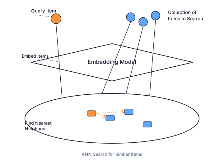
Naive exact KNN: compare against every vector, compute similarity, sort, return top K — O(n). For 1M vectors × 1536 dimensions, that's ~6 billion float ops per query. SIMD/GPU helps, but most apps tolerate slight inaccuracy for big speedups.
def exact_knn(query_vector, all_vectors, k):
    heap = []  # min-heap by similarity
    for vector in all_vectors:
        similarity = compute_similarity(query_vector, vector)
        if len(heap) < k:
            heapq.heappush(heap, (similarity, vector.id))
        elif similarity > heap[0][0]:
            heapq.heapreplace(heap, (similarity, vector.id))
    return sorted(heap, reverse=True)
Approximate Nearest Neighbor (ANN) search trades accuracy for speed — you find probably the nearest neighbors most of the time. Key quality metric: recall — of the true top-K, what fraction did you find? Recall 0.95 means 95% of true neighbors recovered — plenty for most apps.
Indexing strategies
Vector databases make retrieval fast with indexes that skip most comparisons. Tradeoffs are hard to reason about without benchmarking on your data — a major benefit of managed vector DBs is swapping strategies without rewriting your app. You'd use an evaluation set (queries + known-good results) and tune recall vs latency.
HNSW (Hierarchical Navigable Small World)
The most popular production algorithm. Intuition: skip lists. Regular linked list search is O(n). Skip lists add express-lane layers — start at the top, zoom forward until you'd overshoot, drop down, repeat — O(log n).
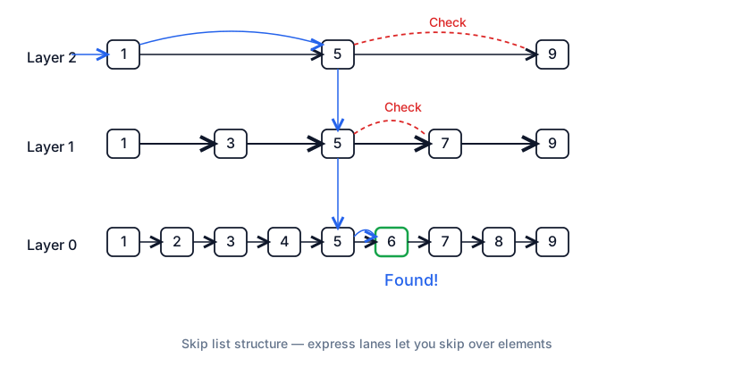
HNSW builds a multi-layer graph. Each vector is a node; edges connect similar vectors. Insert "Taylor Swift" and it links to geometrically nearby embeddings like Beyoncé and Ed Sheeran — no manual curation.
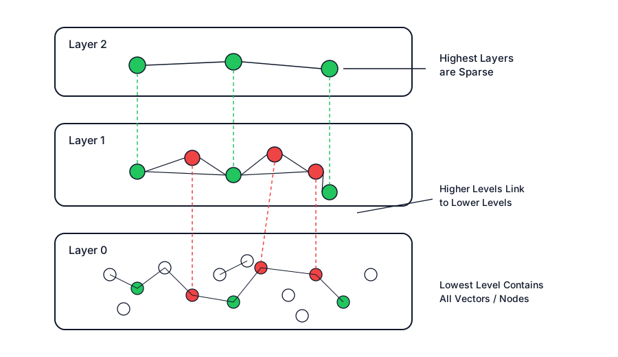
- Start at the top layer with a random entry point.
- Greedy search — move to the neighbor closest to the query.
- Repeat until no improvement at this layer.
- Drop to the next denser layer and continue.
- At Layer 0, thorough local search for final top-K.
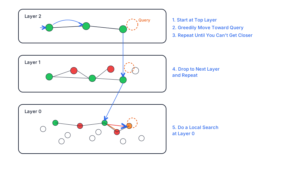
Top layers zoom to the right region; Layer 0 finishes locally. O(log n) with 95%+ recall — why HNSW is the default. Costs: ~2× memory (graph edges + vectors), slow builds, expensive inserts (find place + wire edges at each layer).
IVF (Inverted File Index)
Partition vectors into k-means clusters with centroids. At query time, find nearest centroids, search only those clusters. 1000 clusters, probe 10 → skip 99% of comparisons. Like geospatial indexing, boundary queries need adjacent clusters — in 1536D there are a lot of "edges."
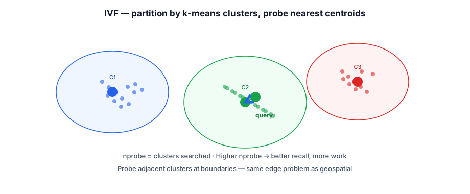
nprobe controls clusters searched. Faster builds, cheaper inserts, often lower recall than HNSW.Locality Sensitive Hashing (LSH)
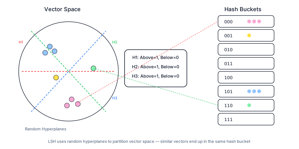
Hash functions designed so similar vectors collide in the same bucket — opposite of regular hashes. Random hyperplanes: each vector is above or below the plane → one hash bit. Eight hyperplanes → 8-bit hash. Multiple hash tables improve recall.
Annoy (Spotify)
Forest of random projection trees — recursively split space with hyperplanes equidistant between random points until leaves hold ~100 vectors. Search traverses toward matching leaves across many trees, union candidates, exact distance on candidates. Killer feature: memory-mapped index — instant load, shared across processes, indexes larger than RAM. Downside: immutable — rebuild to add/remove. Great for static catalogs (music), not real-time streams.
Filtering and hybrid search
Real apps rarely want "top 10 similar" without constraints. You want similar items in stock, in price range, published this year. Two approaches:
- Post-filtering — retrieve top-N (N ≫ K), filter to K. Restrictive filters may not yield K results unless you increase N.
- Pre-filtering — filter first, ANN on the subset. May not use your index efficiently on arbitrary subsets.
How popular systems handle it
- pgvector — Postgres query planner picks vector index, B-tree on filter column, or brute-force on filtered rows. No true filtered HNSW traversal; awkward middle-ground selectivity can get suboptimal plans.
- Elasticsearch — kNN
filterduring graph traversal; restrictive filters mean exploring more of the graph until K matches. Native hybrid: BM25 + vector viasub_searchesor rescore. - Pinecone — metadata filters during ANN; inverted indexes on metadata intersected with vector search. Tunable "filter effort" for latency vs precision.
Hybrid search combines keyword + vector — "red running shoes" matches keywords for color/category while vectors capture semantic related products. Run both in parallel and merge, or use rescore/rank fusion.
Inserts, updates, and index maintenance
Vector DBs are read-optimized. Writes are harder — especially with HNSW. Each insert finds graph placement and updates edges; heavy insert load can degrade graph quality vs a bulk-built index. IVF clusters drift and may need periodic rebuilds.
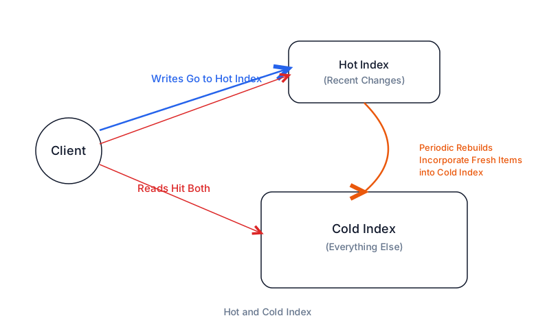
- Updates — usually delete + insert; soft deletes until compaction.
- Rebuilds — HNSW over millions of vectors can take hours. Plan rolling rebuilds, partitioned indexes, or background reindexing.
- Embedding model changes — all old embeddings incompatible; re-embed everything or maintain parallel indexes during migration.
Vector database options
The field moves fast. Practical advice: start simple. You probably don't need a purpose-built vector DB — extensions on Postgres or Elasticsearch handle millions of vectors and avoid another operational surface. Reach for dedicated vector DBs when scale or features demand it (~100M+ vectors is a common threshold).
Extensions (start here)
| Option | When |
|---|---|
| pgvector | Already on Postgres — HNSW + IVF, joins with relational data, ACID. "Similar products in stock in user's region" in one query. |
| Elasticsearch kNN | Already running ES — hybrid BM25 + vector out of the box. |
| Redis Vector Search | Need sub-ms latency; simpler indexes, often enough. |
| S3 Vectors (AWS) | Vectors in S3, query via S3 API — minimal new infra if you're S3-native. |
Purpose-built (scale)
| Option | Tradeoff |
|---|---|
| Pinecone | Fully managed serverless API — easiest ops, higher cost, less control. |
| Weaviate | Open source, GraphQL, strong hybrid search — middle ground. |
| Milvus | Billions of vectors — serious distributed ops. |
| Qdrant | Rust, excellent filtered search. |
| Chroma | Lightweight — popular for RAG prototyping. |
Using vector databases in your interview
Vector DBs show up in AI/ML-adjacent designs — you'll usually know going in. Common scenarios:
- Semantic search — document/code search with natural language queries.
- Recommendations — items similar to what the user engaged with (+ collaborative filtering).
- Image/video similarity — reverse image search, similar videos.
- RAG — retrieve relevant chunks, LLM synthesizes answer.
- Deduplication — near-duplicate detection (plagiarism, duplicate listings).
- Anomaly detection — embeddings far from normal patterns (fraud).
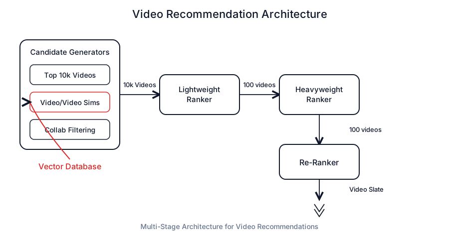
Architecture patterns
- Vector DB as separate service — embed query → ANN → IDs → primary DB for full records. Clean separation. Default for most interviews.
- Hybrid search — parallel keyword + vector, merge rankings.
- Two-stage retrieval — ANN top-1000 → slow reranker with rich features.
Decisions to discuss
- Consistency — vector search can be eventually consistent; new items searchable after seconds/minutes is OK.
- Update strategy — real-time embed on create vs hourly batch job.
- Filtering — pre vs post vs integrated; depends on selectivity.
- Index type — "HNSW for query performance" unless write-heavy or memory-bound.
- Embedding model — mention sentence transformers or OpenAI API; tag which model version produced each vector.
Numbers to know
| Metric | Ballpark |
|---|---|
| Embedding dims | 128–1536 typical (OpenAI 1536; open-source 384/768) |
| Memory per vector | 4 bytes/dim float32 → ~6KB for 1536-dim raw |
| 1M vectors @ 1536 | ~6GB vectors; HNSW ~2× with graph overhead |
| Query latency | 1–10ms well-tuned; sub-5ms common in-memory |
| Recall target | 95%+ usually OK; 99%+ costs latency/memory |
| Throughput | Tens of thousands QPS/node on in-memory indexes |
Cost and performance levers
ANN interview sketch
Filter + ANN
Pre-filter vs post-filter: selective ACL should pre-filter or use metadata-aware indexes; post-filter can return too few results after top-k.
Failure modes to mention
Call out at least one dependency failure (DB down, cache stampede, queue lag, region outage) and your mitigation (timeouts, retries with jitter, degraded mode, circuit breaker).
Interview Q&A by level
Practice saying these out loud for vector databases. Interviewers grade clarity and judgment more than buzzwords.
Match depth to the bar: define → trade off → operate. Don't dump principal answers in an entry-level screen.
Wrapping up
Vector databases enable applications built on semantic similarity rather than exact matching. The core is ANN search — HNSW is the production default. Start with pgvector or Elasticsearch kNN; graduate to purpose-built DBs when extensions can't keep up.
In interviews: know the problem (find similar things fast), the mechanism (embeddings + ANN), and when it's the right tool (semantic search, recommendations, RAG — not exact ID lookup). Stick with Pattern 1 architecture unless the prompt demands ranking depth.
Continue with RAG, Elasticsearch, PostgreSQL, Prompt engineering, Key technologies, and Common patterns.