Why proximity keeps showing up
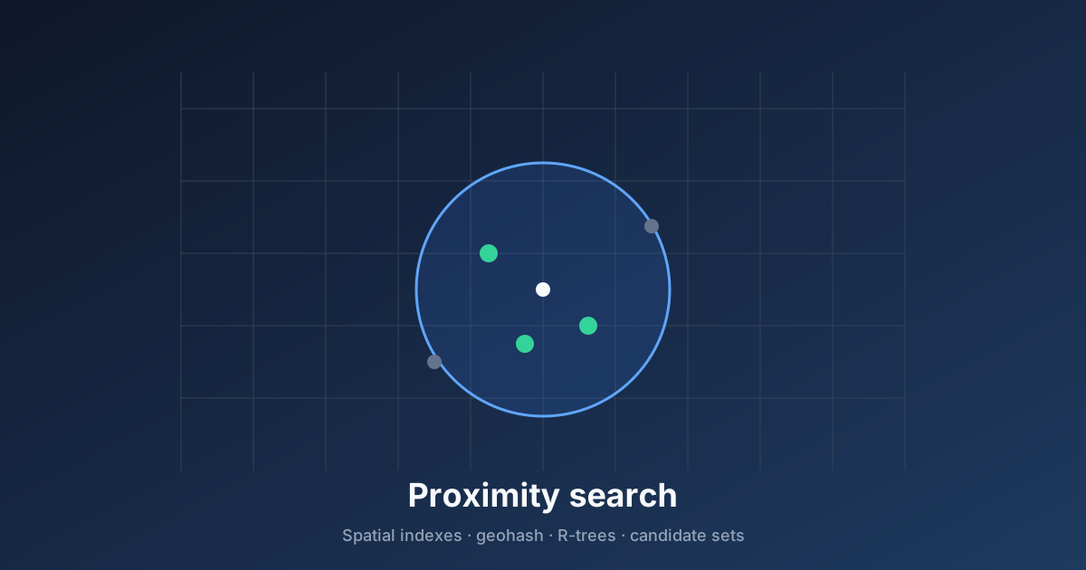
Proximity search is one of those oddly specific topics that's somehow become a regular in system design interviews. It shows up anytime you're searching by location instead of by ID or value — drivers near a rider, restaurants near a user, people near a place.
Lat/lng B-trees ≠ nearby.
Quadtree · BKD · R-tree.
Geohash · S2 · H3.
Candidates → Haversine.
Why a B-tree finds ages but not drivers
At first glance this doesn't seem hard — databases are great at sorting. Ask for every user between ages 20 and 25 and it returns in milliseconds. So why doesn't "every driver within 2 km of a rider" work the same way? Same database, same volume of data — one query is instant, the other becomes a full table scan.
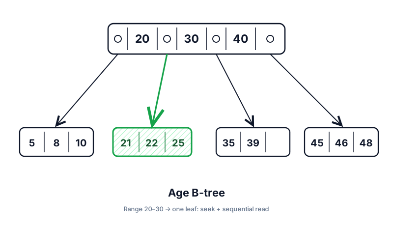
The age query is fast because a B-tree keeps sorted keys packed together on disk. 20 sits next to 21 next to 22 on the same page — "everyone between 20 and 30" is one seek plus a short sequential read.
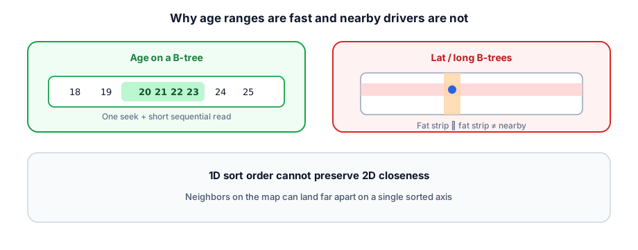
Location doesn't work the same way. You have two numbers — latitude and longitude — and what you care about is geodesic distance on a sphere. A single B-tree only sorts one of those numbers. Index latitude → horizontal strip of Earth. Index longitude → vertical strip. Even a composite (lat, lng) index sorts by the first column and breaks ties with the second, so you still pull a fat strip of millions of rows, none ranked by distance from the rider.
-- Looks sensible. Falls apart for "within 2km of me."
CREATE INDEX idx_drivers_lat ON drivers(lat);
CREATE INDEX idx_drivers_lng ON drivers(lng);

-- Planner may use both indexes (bitmap AND) → still a huge
-- lat band ∩ lng band, then filter EVERY survivor:
SELECT * FROM drivers
WHERE lat BETWEEN :lat - d AND :lat + d
  AND lng BETWEEN :lng - d AND :lng + d
AND haversine(lat, lng, :lat, :lng) <= 2000;Distance math you actually need
Interviewers occasionally push "how do you compute distance?" You don't need a geodesy degree — you need to know which formula belongs where.
| Formula | Cost | Use when |
|---|---|---|
| Equirectangular / planar | Cheapest (Δlat, Δlng × cos) | Tiny radii (< few km), candidate pre-filter only |
| Haversine | Moderate (trig on sphere) | Default post-filter for city-scale radius queries |
| Vincenty / Karney | Expensive, ellipsoidal | Survey / aviation accuracy — almost never interviews |
| Road / ETA | Routing graph (OSRM, Google) | "Nearest driver" for matching — after geo candidates |
import math

def haversine_m(lat1, lon1, lat2, lon2):
    R = 6_371_000  # mean Earth radius
    p1, p2 = math.radians(lat1), math.radians(lat2)
    dp = math.radians(lat2 - lat1)
    dl = math.radians(lon2 - lon1)
    a = (math.sin(dp / 2) ** 2
         + math.cos(p1) * math.cos(p2) * math.sin(dl / 2) ** 2)
return 2 * R * math.asin(math.sqrt(a))Two approaches — trees vs encoded keys
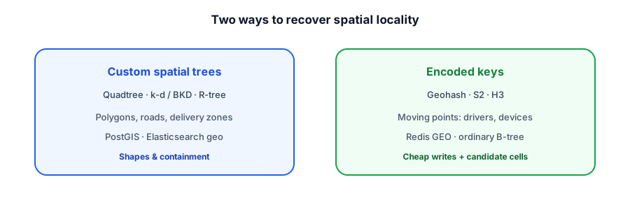
- Custom spatial trees — polygons, roads, delivery zones, containment and intersection. PostGIS (GiST/R-tree), Elasticsearch BKD geo.
- Encoded keys — points that move constantly. Flatten lat/lng into one sortable key: Redis GEO (geohash int), geohash strings, S2, H3 on a normal B-tree / sorted set.
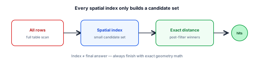
Query shapes you'll name: radius (within R meters), kNN (k nearest), bbox (map viewport), contains (point in polygon). Trees shine at contains/intersection; encoded keys shine at radius/kNN on churning points.
Custom trees: quadtrees
The first approach builds a purpose-made tree for spatial data. On disk, survivors of this lineage are shaped to behave like a B-tree — balanced, page-sized nodes, predictable depth. Each structure below fixes a problem the previous one couldn't.
The quadtree is still the cleanest intuition builder. Turn the map into a tree: the whole map is the root; split into four equal quadrants; any quadrant that holds more than capacity k points splits again. Points live in the leaves. Search: walk from the root comparing your query to each cell's midpoint until you hit a leaf — that leaf plus neighbors form the candidate set.
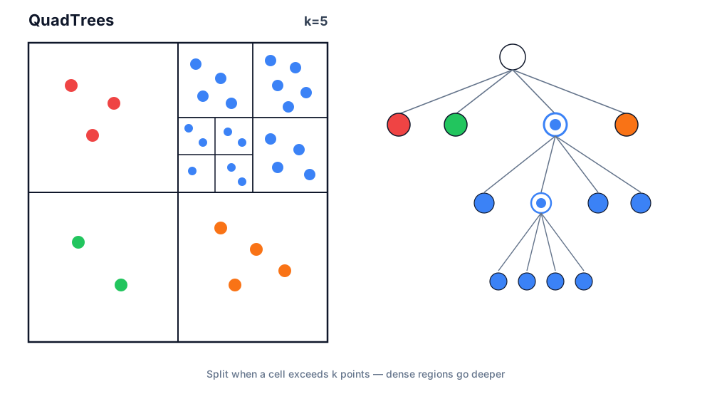
- Variants — point quadtrees (points in nodes) vs region/PR quadtrees (points only in leaves; what interviews mean).
- Strength — adapts to density (Manhattan deep, empty lake shallow).
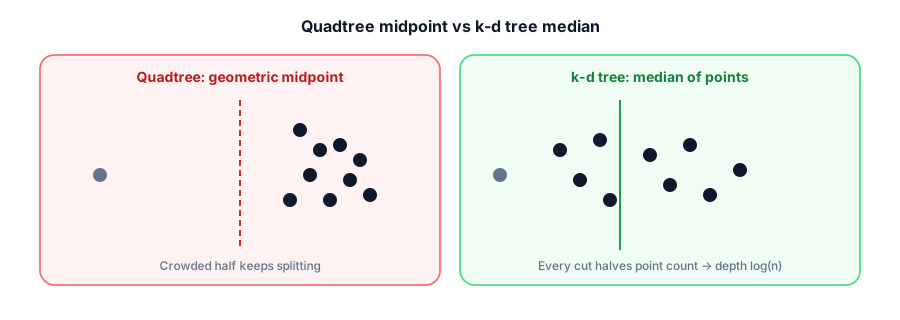
- Depth problem — geometric midpoints, so dense clusters burn many levels; p99 depends on where you look.
- Disk problem — pointer-heavy; each hop risks a random page read once you leave RAM.
Still everywhere in memory: Google Maps tile pyramids, game-engine collision, image compression. For a durable DB index that stays fast past RAM, you need something sturdier.
k-d trees and BKD trees
A k-d tree is the binary cousin. Instead of splitting on every dimension at once, it alternates axes: level 1 on x, level 2 on y, level 3 on x. Split at the median of points (not the geometric midpoint) and depth stays ~log₂(n) even when density is lopsided.
Classic k-d trees inherit the pointer / disk problem. The modern fix is the BKD tree (block k-d tree, from papers behind Lucene): pack many points into disk-page-sized blocks, build from a sorted batch, keep fanout high like a B-tree. Great for relatively static geo documents. Painful for drivers that move every second — rebuild cost dominates.
R-trees and PostGIS
The R-tree was built from the ground up for on-disk databases and fixed two gaps earlier trees left open: shapes (lines, polygons) and mutating data with B-tree-like page splits.
Wrap every object in a minimum bounding rectangle (MBR) — axis-aligned box. Nearby rectangles nest inside larger ones up to the root. Leaves sit at the same depth; nodes fit a disk page; inserts/deletes split and merge like a B-tree.
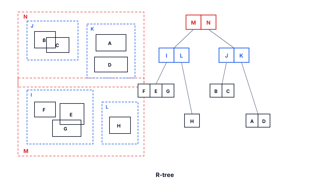
Rectangles can overlap. Query lands in two boxes → descend both. Production ships R*-tree insertion heuristics (minimize overlap and margin) — what almost every modern implementation uses under the hood.
-- PostGIS on Postgres (GiST ≈ R-tree behavior)
CREATE EXTENSION postgis;

ALTER TABLE zones ADD COLUMN geom geography(POLYGON, 4326);
CREATE INDEX zones_gix ON zones USING GIST (geom);

-- Point-in-polygon / containment
SELECT id FROM zones
WHERE ST_Contains(geom, ST_SetSRID(ST_MakePoint(:lng, :lat), 4326));

-- Radius (geography uses meters on spheroid)
SELECT id, ST_Distance(loc, rider) AS meters
FROM drivers
WHERE ST_DWithin(loc, ST_SetSRID(ST_MakePoint(:lng, :lat), 4326)::geography, 2000)
ORDER BY loc <-> ST_SetSRID(ST_MakePoint(:lng, :lat), 4326)
LIMIT 20;Encoded keys — reuse a normal index
Spatial trees work, but they need special index/query code and often a spatial extension. The encoded-key approach skips the custom tree: turn lat/lng into a cell ID or sortable key that an ordinary B-tree or sorted set already understands. A moving driver becomes one integer/string update — the shape you want at millions of writes/sec.
Under the hood most encodings are space-filling curves (Morton / Z-order for geohash, Hilbert variants in some systems): interleave bits of x and y so 2D neighbors usually share a long common prefix on the 1D line.
Geohash
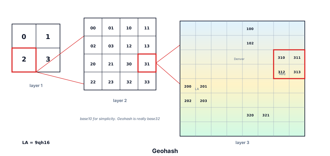
Geohash turns space-filling-curve math into something you can compute in a few lines. Divide the world into a base-32 grid; each character zooms into one of 32 subcells. Longer string → finer cell.
| Length | ~Cell size | Interview use |
|---|---|---|
| 4 | ~40 km | City / region shard key |
| 5 | ~5 km | Coarse nearby |
| 6 | ~1.2 km | Neighborhood |
| 7 | ~150 m | Dense urban matching |
| 8–9 | ~20–5 m | Parking / precise pin |
-- Ordinary B-tree on encoded cell
CREATE INDEX drivers_geohash ON drivers (geohash);

-- Prefix scan + exact distance post-filter
SELECT id FROM drivers
WHERE geohash LIKE 'dr5ru%'
  AND haversine_m(lat, lng, :lat, :lng) <= 2000;
# Redis: GEOADD stores a 52-bit geohash as a sorted-set score
GEOADD drivers -73.9857 40.7484 driver:42
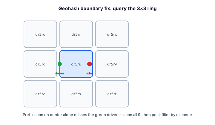
GEOSEARCH drivers FROMLONLAT -73.98 40.75 BYRADIUS 2 km WITHDIST ASC COUNT 20Catch: cell boundaries. Two points a meter apart can get unrelated prefixes if they straddle an edge. Fix: the 3×3 (or 3×3×depth) trick — query your cell plus eight neighbors, then post-filter by exact distance.
S2 and H3
Google S2 wraps the globe in a cube, projects onto six faces, and assigns 64-bit hierarchical cell IDs (Hilbert curve per face). Truncate bits to get a parent cell. Roughly equal area, handles antimeridian wrap, underpins MongoDB's 2dsphere index and much of Google Maps.
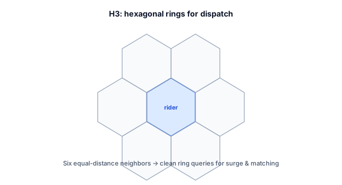
Uber H3 uses hexagons. A square has four edge neighbors and four farther corner neighbors — messy for rings and heat maps. A hexagon has six neighbors at roughly equal distance. Cells are 64-bit hierarchical IDs, but H3 does not lay them on a space-filling curve for range scans — you compute the ring of IDs and WHERE h3_cell IN (...).
# Pseudocode — Uber-style candidate generation
rider_cell = h3.latlng_to_cell(lat, lng, res=9)  # ~100–200m
cells = h3.grid_disk(rider_cell, k=2)           # center + 2 rings
candidates = db.query(
    "SELECT * FROM drivers WHERE h3_cell = ANY(%s) AND updated_at > now() - interval '30s'",
    [list(cells)],
)
ranked = sorted(candidates, key=lambda d: eta(d, rider))[:5]| Geohash | S2 | H3 | |
|---|---|---|---|
| Shape | Rectangles | ~Equal-area cells on sphere | Hexagons |
| Curve / lookup | Z-order → prefix/range | Hilbert → prefix/range | Explicit ring math |
| Best for | Simple city apps, Redis | Global / spherical correctness | Dispatch, surge, analytics rings |
| Seen in | Redis GEO, DIY B-trees | MongoDB 2dsphere, Google | Uber |
Production architecture — rides & delivery
A whiteboard that stops at "Redis GEO" is junior. A senior design separates write path, read/match path, and shard boundaries.
- Shard by city / metro first — never run a global geo query for a 2 km ride. Koramangala traffic must not scan Delhi drivers.
- Driver heartbeats — phone pings every 3–10s: update lat/lng + cell ID in an in-memory store (Redis). TTL /
updated_atdrops stale positions. - Match — encode rider cell → ring of cells → candidate set → filter online + fresh → rank by ETA → offer.
- Zones & geofences — surge polygons, no-pickup airports: PostGIS / S2 polygons offline; cache compiled cells for the hot path.
- Durable copy — Postgres/Cassandra for trips and history; Redis is the matching hot set, not the system of record.
Driver phone
   │  GPS ping (3–10s)
   ▼
Ingest / API  ──►  Redis GEO or H3 hash  (city shard)
                      │
Rider request ───────►│  GEOSEARCH / cell IN ring
                      ▼
                 Candidates → Haversine → ETA service
                      │
                      ▼
Offer / dispatch · write trip to Postgres- Stale GPS — require
updated_atwithin N seconds; otherwise treat as offline. - Clock skew — server receive time beats device clock for freshness.
- Privacy — store coarse cells for analytics; fine coordinates only for active trips.
- Map viewport — bbox query for "restaurants on screen" ≠ radius kNN for matching; say which one you mean.
Which should you use?
| Choose | When | Stack | Watch out |
|---|---|---|---|
| Spatial tree | Polygons, roads, zones, contains / intersects | PostGIS GiST, ES BKD geo_shape | Heavier writes; BKD write-once segments |
| Encoded cells | Points that move constantly | Redis GEO, geohash+B-tree, S2, H3 | Ring queries + post-filter; mostly points |
| Hybrid | Real dispatch platforms | Redis/H3 hot path + PostGIS zones | Two systems to keep consistent |
Cost and performance levers
In your interview
What to say out loud
"I won't B-tree lat and lng separately — that gives strips, not nearby. I'd shard by city, keep live drivers in Redis GEO or H3 cells with a freshness TTL, query the cell plus neighbors, Haversine-filter, then rank by ETA. Delivery zones and geofences live in PostGIS. Surge is density per cell — hex rings make that clean."
- Name the failure of 1D indexes before naming a product.
- Separate matching hot path from durable trip storage.
- Call out boundary rings, stale GPS, and hot cells / surge.
- Don't invent a custom quadtree on the whiteboard unless asked — name the production default.
Geo interview sketch
Redis GEO one-liner
GEOADD/GEOSEARCH is a fine interview default for "nearby drivers" before introducing ES geo or S2 cells.
Failure modes to mention
Call out at least one dependency failure (DB down, cache stampede, queue lag, region outage) and your mitigation (timeouts, retries with jitter, degraded mode, circuit breaker).
Interview Q&A by level
Practice saying these out loud for proximity / geo search. Interviewers grade clarity and judgment more than buzzwords.
Match depth to the bar: define → trade off → operate. Don't dump principal answers in an entry-level screen.
Wrapping up
Proximity search recovers 2D locality that a 1D index destroys. Custom trees (quadtree → k-d/BKD → R-tree) understand shapes and disk pages. Encoded keys (geohash, S2, H3) reuse ordinary indexes for moving points. Both only generate candidates — Haversine (and often ETA) finishes the job. Shard by city, keep the hot path in memory, and treat PostGIS as the geometry brain rather than the heartbeat sink.
Continue with Design Yelp, Database indexing, Redis geospatial, PostGIS / Postgres, Elasticsearch geo, and the proximity services pattern.