Why DynamoDB
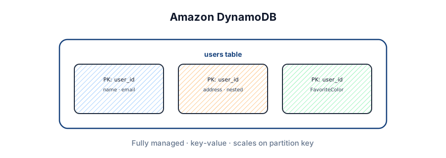
DynamoDB is a fully managed, highly scalable key-value service from AWS. Buzzwords — but what do they mean?
- Fully managed — AWS handles hardware, patching, configuration, and scaling. You focus on application code.
- Highly scalable — handles massive data and traffic; auto-scales without downtime or performance cliffs.
- Key-value — NoSQL, not relational. Flexible item storage keyed by a primary key you choose.
For system design interviews, DynamoDB has just about everything you'd need from a database — including ACID transactions across up to 100 items. That neutralizes the old "NoSQL means no transactions" criticism.
Table · item · attributes.
Partition + optional sort.
Query · GSI/LSI · no scans.
Cost · vendor lock-in · modeling.
The data model
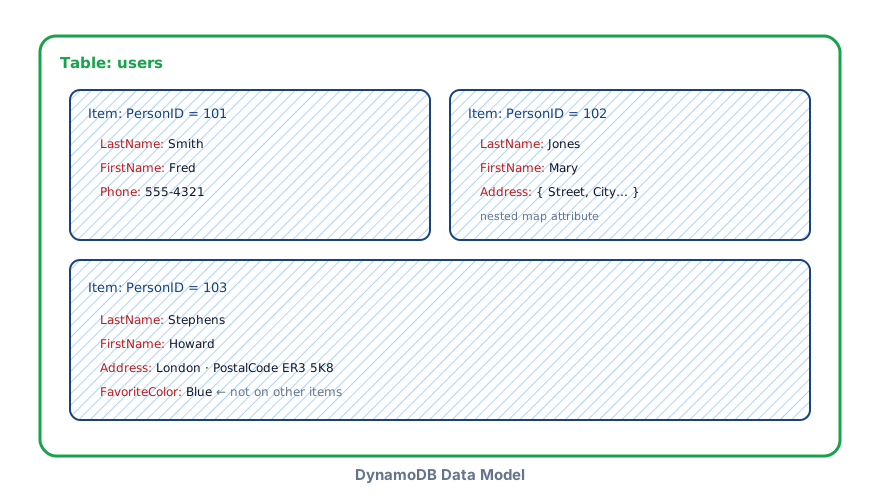
Data lives in tables of items made of attributes — familiar names, but tuned for scale and flexibility.
- Tables — top-level structure; mandatory primary key; support secondary indexes.
- Items — like rows; up to 400 KB each including all attributes.
- Attributes — key-value pairs; scalar, set, or nested; sparse across items.
{
  "PersonID": 101,
  "LastName": "Smith",
  "FirstName": "Fred",
  "Phone": "555-4321"
},
{
  "PersonID": 102,
  "LastName": "Jones",
  "FirstName": "Mary",
  "Address": {
    "Street": "123 Main",
    "City": "Anytown",
    "State": "OH",
    "ZIPCode": 12345
  }
},
{
  "PersonID": 103,
  "LastName": "Stephens",
  "FirstName": "Howard",
  "Address": { "Street": "123 Main", "City": "London", "PostalCode": "ER3 5K8" },
  "FavoriteColor": "Blue"
}
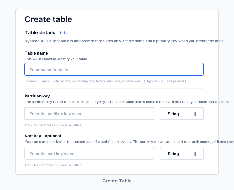
JSON is the wire format — storage underneath is proprietary. Create tables in the AWS console and start inserting immediately; no upfront schema migration.
Partition key and sort key
Every table has a primary key — one or two attributes that uniquely identify each item.
- Partition key — hashed to determine physical storage location.
- Sort key (optional) — combined with partition key for composite key; enables range queries and sorting within a partition.

For a group chat app, use chat_id as partition key and message_id as sort key — fetch all messages for one chat, sorted chronologically. Prefer a monotonically increasing ID over a raw timestamp: timestamps don't guarantee uniqueness when multiple messages land in the same millisecond.
- Auto-incrementing counters per partition
- UUID v7 (sortable, no MAC leak like v1)
- Snowflake IDs
- ULID
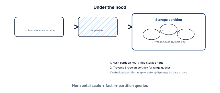
Under the hood: a request router consults a centralized partition metadata service (conceptually similar to consistent hashing, but managed by AWS). Within each partition, items are organized in a B-tree indexed by sort key. Composite-key queries hash to the right node, then traverse the B-tree.
Secondary indexes
Need to query by an attribute that isn't your partition key? Add a secondary index.
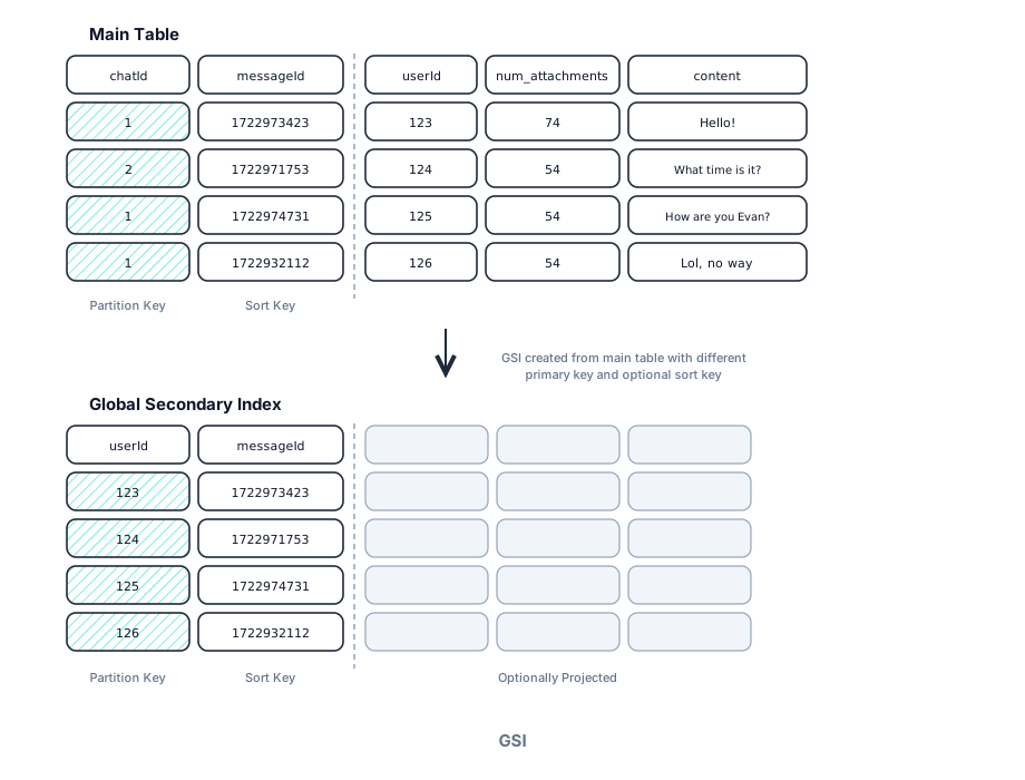
Global Secondary Index (GSI)
Different partition key (and optional sort key) from the base table. Data lives on entirely separate physical partitions, replicated asynchronously. Use when you need cross-partition queries — e.g. all messages by user_id when the base table is keyed by chat_id.
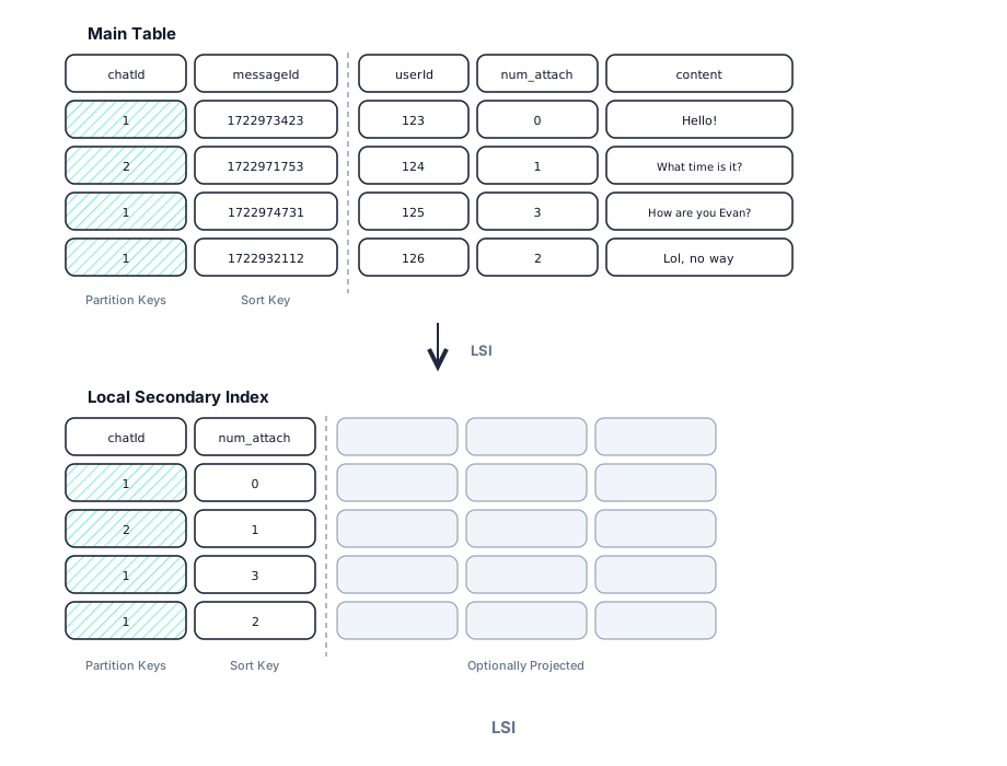
Local Secondary Index (LSI)
Same partition key as the base table, different sort key. Co-located on the same physical partitions — efficient for range queries within a partition. Example: sort messages by num_attachments within one chat. Caveat: LSIs must be defined at table creation and cannot be added later.
| Feature | GSI | LSI |
|---|---|---|
| Partition key | Different from base table | Same as base table |
| When to use | Query non-primary-key attributes globally | Additional sort within same partition |
| Size limit | No index item size restriction | 10 GB per partition key |
| Throughput | Separate RCU/WCU | Shares base table capacity |
| Consistency | Eventually consistent only | Eventual or strong reads |
| Lifecycle | Add/remove anytime | Define at creation; cannot remove |
| Max count | 20 per table | 5 per table |
GSIs are separate internal tables updated asynchronously. LSIs maintain a separate B-tree per partition, updated synchronously with base-table writes.
Accessing data
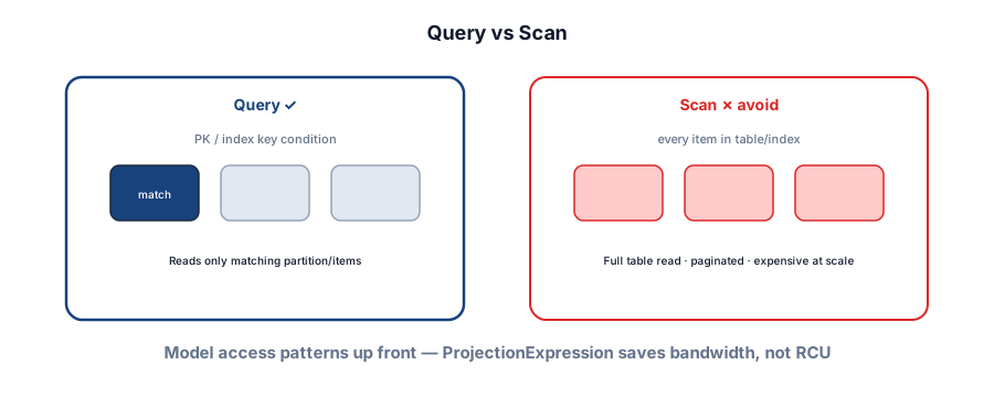
Two primary operations: Query (efficient) and Scan (avoid at scale).
- Query — reads items matching primary key or index key conditions; supports sort-key ranges.
- Scan — reads every item in a table or index; paginated; expensive on large datasets.
// SQL: SELECT * FROM users WHERE user_id = 101
const params = {
  TableName: 'users',
  KeyConditionExpression: 'user_id = :id',
  ExpressionAttributeValues: { ':id': 101 }
};
dynamodb.query(params, callback);

// SQL: SELECT * FROM users  →  avoid at scale
const scanParams = { TableName: 'users' };
dynamodb.scan(scanParams, callback);
DynamoDB's primary interface is the AWS SDK (or PartiQL as a SQL-compatible layer — same operations underneath). Reads return the full item by default. ProjectionExpression trims the response over the wire but still charges RCUs on the full item size — unlike SQL column projection.
CAP and consistency
Match your database to non-functional requirements early. DynamoDB isn't "always AP" anymore — consistency is chosen per read request, not per table. See CAP theorem and Consistency models.
- Eventual consistency (default) — highest availability, lowest latency; may not see the latest write immediately.
- Strong consistency — set
ConsistentRead=trueon GetItem/Query/Scan; 2× RCU cost; reflects all prior successful writes.
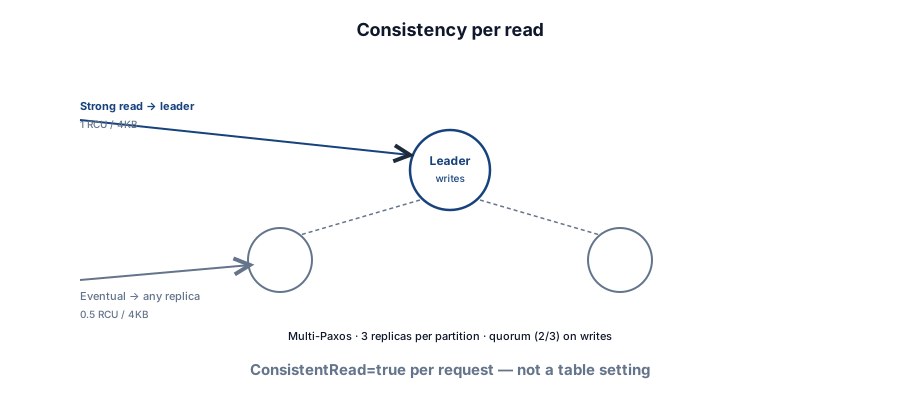
Each partition runs a leader-based replication group of three nodes (Multi-Paxos). Writes go through the leader; quorum (2/3) persists the WAL before ack. Strong reads hit the leader; eventual reads can use any replica.
Transactions — TransactWriteItems and TransactGetItems provide serializable isolation across up to 100 items in multiple tables. Strong consistent reads work on base tables and LSIs only — not GSIs.
Architecture and scalability
DynamoDB auto-shards when a partition hits size or throughput limits. Hash-based partitioning spreads load; AWS replicates each partition across three Availability Zones in a region (not user-configurable).
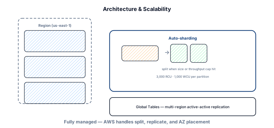
Global Tables — active-active multi-region replication for local reads/writes worldwide. In interviews, mentioning Global Tables for cross-region apps is often enough.
Fault tolerance and security
Three replicas per partition across AZs provide durability and availability during hardware or network failures. Cross-region durability requires Global Tables.
- Encryption at rest by default
- TLS enforced for all API calls
- IAM fine-grained access control
- VPC endpoints for private access without public internet
Cost and performance levers
DynamoDB bills on throughput units, not servers. Two modes: on-demand (per request) and provisioned (hourly RCU/WCU with auto scaling).
| Unit | Throughput | On-demand (approx.) |
|---|---|---|
| RCU | 4 KB read/sec (1 strong or 2 eventual) | ~$1.12 / million reads |
| WCU | 1 KB write/sec (rounded up) | ~$5.62 / million writes |
Advanced features
DAX (DynamoDB Accelerator)
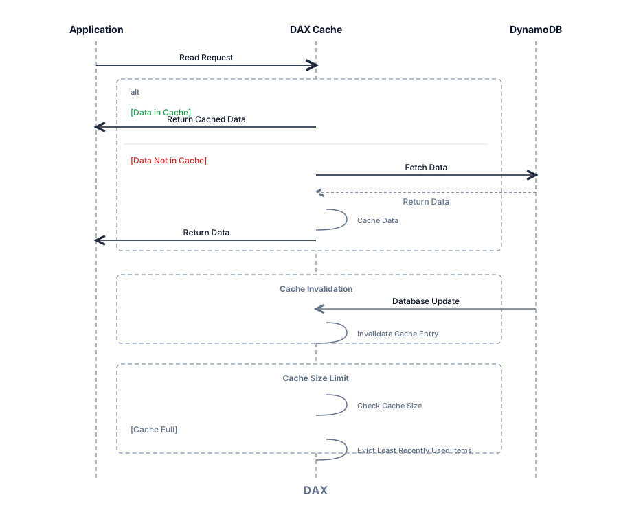
Purpose-built in-memory cache — microsecond reads for hot paths. Swap the DynamoDB client for the DAX SDK (Java, .NET, Node, Python, Go). Read-through and write-through; item cache + query cache always active. Caveats: writes that bypass DAX leave stale cache until TTL; strong reads aren't cached.
DynamoDB Streams
Built-in CDC — every insert, update, and delete becomes a stream record for downstream consumers.
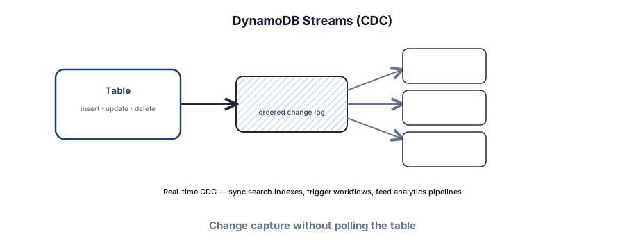
- Search sync — Streams → Lambda → Elasticsearch index
- Real-time analytics — enable Kinesis on the table, then Firehose to S3/Redshift/OpenSearch
- Change notifications — Streams → Lambda for cache invalidation or webhooks
DynamoDB in an interview
When to use it
- High availability and horizontal scale on AWS.
- Clear upfront access patterns — key-value or document shapes.
- Single-digit ms latency; microsecond with DAX.
- Transactions, Streams, and Global Tables cover many "but what about…" objections.
When not to
- Extreme write volume where per-request pricing dominates (do the RCU/WCU math).
- Complex joins, ad-hoc aggregations, or constantly new query shapes.
- You're stacking GSIs/LSIs because access patterns weren't designed — consider Postgres.
- Interviewer wants vendor-neutral designs — compare with Cassandra or self-managed alternatives.
Single-table sketch
Cost gotcha
Scans and over-provisioned capacity burn money. Design for Query; use on-demand for spiky unknown workloads; watch GSI projection size.
Failure modes to mention
Call out at least one dependency failure (DB down, cache stampede, queue lag, region outage) and your mitigation (timeouts, retries with jitter, degraded mode, circuit breaker).
Interview Q&A by level
Practice saying these out loud for DynamoDB. Interviewers grade clarity and judgment more than buzzwords.
Match depth to the bar: define → trade off → operate. Don't dump principal answers in an entry-level screen.
Wrapping up
DynamoDB is versatile and interview-friendly when your interviewer allows AWS. Its value shows up when partition keys, GSIs, and per-request consistency match your access patterns — not when you need relational flexibility you didn't model for.
Compare with PostgreSQL (interview default), Apache Cassandra (open-source, query-driven wide-column), MongoDB (document store), Data modeling (when to pick SQL vs NoSQL), and Key technologies for the broader crew roster.
How to answer this in a backend interview
I'd only pick DynamoDB after listing access patterns. Partition key spreads load; sort key supports 'all orders for user by time.' I'd design a single-table layout or a few tables intentionally, and add GSIs only for real alternate paths. Reads are eventually consistent by default — I'd call for strongly consistent only where the product breaks without it. Capacity is either on-demand or provisioned with autoscaling; hot partitions are the failure mode I name out loud.
Related Lattice posts: Data modeling · Cassandra · Sharding · Caching strategies